![]()
![]()
![]()
Use LEFT and RIGHT arrow keys to navigate between flashcards;
Use UP and DOWN arrow keys to flip the card;
H to show hint;
A reads text to speech;
37 Cards in this Set
- Front
- Back
- 3rd side (hint)
|
Average tax rate |
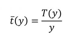
average rate at which an individual or corporation is taxed |
|
|
|
Marginal tax rate |
|
|
|
|
Proportional tax rate |
T(y) = τ • y |
|
|
|
Allocative perspective of taxation policy - fostering efficiency |
- Maximize the "size of the cake" - State interventions in case of market failures, notably - Public goods (e.g., national defense) - Externalities - Stimulate activities beneficial to society and - Discourage activities costly to society |
|
|
|
Distributive perspective of taxation policy |
- Individuals differ in endowments (inc. abilities), resulting in unequally distributed market outcomes (income, wealth, abilities to consume) - Reduce inequalities in market outcomes |
|
|
|
First theorem of welfare economics |
Under local nonsatiation of preferences, a Walras equilibrium is Pareto efficient. Requirements: 1. Completeness - No transactions costs and because of this each actor also has perfect information 2. Price-taking behavior - No monopolists and easy entry and exit from a market. 3. Absence of market failures (information asymmetries, externalities, public goods)Under these conditions, there is no allocative but only a distributional argument for state interventions (Adam Smith's "invisible hand"). |
3 |
|
|
Second theorem of welfare economics |
Out of all feasible Pareto optimal allocations, one can achieve any particular one by enacting a lump-sum tax and then letting the market take over.
Additional requirements to the first theorem of welfare economics: convexity of preferences and production set. |
|
|
|
Linear tax schedule ("negative income tax" when b>0) |
T(y) = τ • y - b τ>0 |
|
|
|
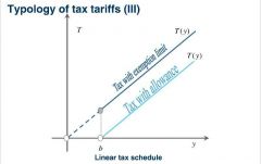
Tax with an allowance |
T(y) = max {τ • (y - b), 0} τ, b > 0 |
|
|
|
Tax with exemption limit* |
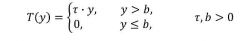
* disadvantage: Reversal of rank order near the limit |
|
|
|
Graphical explanation of the difference between tax exemption limits and allowances |
|
|
|
|
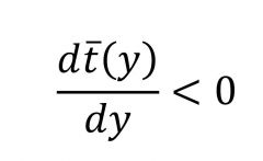
When is a tax progressive? |
A tax is progressive, if an individuals average tax rate increases with income
Progressive tax schedules imply higher marginal tax rates than average tax rates. |
|
|
|
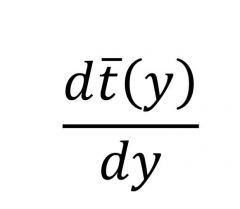
Degree of progressiveness (formula) |
|
|
|
|
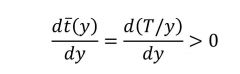
Progressiveness: When is a tax regressive? |
|
|
|
|
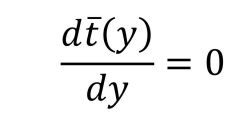
Progressiveness: When is a tax proportional? |
|
|
|
|
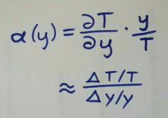
Progressiveness Elasticity of revenue |
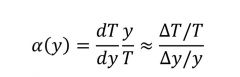
α >1: tax schedule with elastic revenue |
|
|
|
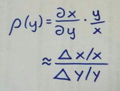
Progressiveness
Residual income elasticity |
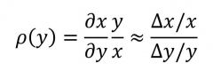
with net income, x(y) = y −T(y) 1. Measure of local progressivity, showing how a marginal variation of pre-tax income changes post-tax income. 2. Progressive tax schedules imply a residual income elasticity of ρ< 1.3. The smaller is ρ, the more progressive the tariff. |
|
|
|
Prototypes of tax schedules for married couples Household taxation: |
|
|
|
|
Prototypes of tax schedules for married couples: Individual taxation: |
|
|
|
|
Prototypes of tax schedules for married couples: Splitting |
|
|
|
|
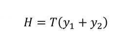
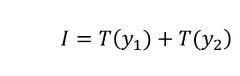
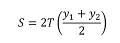
Principles for the taxation of couples |
Non-discrimination of marriage: · The tax burden of two individuals with incomes y1 und y2 should not increase when they get married.
Global income taxation: · The tax burden of the married couple should depend exclusively on the sum y1 + y2 and not on the istribution of the partners' incomes. · Justification: View of married couples as economical distribution(e.g., social welfare benefits, maintenance obligations). |
|
|
|
Taxation of married couples What is the problem with household taxation? |
household taxation violates the non- discrimination principle (Verheiratete Paare zahlen mehr Steuern als unverheiratete) |
|
|
|
Taxation of married couples What is the problem with individual taxation? |
If two spouses have different incomes and the tax is individual and progressive, then they pay a higher tax than a couple where the incomes of both spouses are the same.
Hence, we have a violation of the principle of global income taxation. |
|
|
|
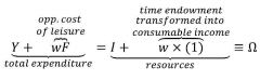
Setup of the labor supply model
Individual utility function + Budget and time restraint |
U(Y,F) = U (Y, 1-L)
Hours of Work: 0 <= L <=1 wage rate: w Time budget: 1 exogenous income: I Leisure time F: 1 - L
Budget constraint: Y = wL + I Time constraint: 1 = L + F |
|
|
|
Setup of the labor supply model
Was folgt aus Budget und time restraint? |
|
|
|
|
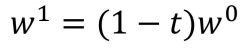
Taxing labor income Disposable income |
Y = I + (1-t)w°L
With: w° gross wage I exogenous income |
|
|
|
Taxing labor income Net wage |
|
|
|
|
Taxing labor income Calculating the tax liability |

= gross income - net income |
|
|
|
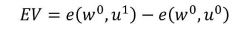
Taxing labor income Dead weight loss |
aka.: excess burden (due to substitution effect) DWL = - EV - R EV Equivalent Variation of the individual welfare loss R Tax Liability |
|
|
|
Taxing labor income Equivalent variation of the individual welfare loss |
|
|
|
|
Taxing labor income Distortionary tax |
Distortionary tax · Changes the relative price of labor. · Substitution effect lowers tax revenues in comparison to the lump-sum tax. · Tax revenues are not sufficiently high to completely compensate the households by reimbursement. · The net loss is the deadweight loss. |
|
|
|
Taxing labor income Lump-sum tax |
Lump-sum tax · Does not change relative prices (parallel shift of budget line), so that no substitution effect is caused. · A reimbursement of the tax revenues would reestablish the original position of the household without loss of utility. |
|
|
|
Elasticity of revenue |
|
|
|
|
Residual income elasticity |
net income x = y - T(y) |
|
|
|
Optimal income taxation
What determines the distributional effects? |
tax liability function T(Y), or likewise the average tax rates T(Y)/Y |
|
|
|
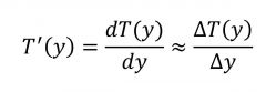
Optimal income taxation
What determines the efficiency effects? |
marginal tax rates T'(Y) |
|
|
|
Optimal income taxation What determines the incentives in the respective income classes? |
Marginal tax rates T'(Y) |
|