Reading...
![]()
Play button
![]()
Play button
![]()
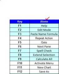
Use LEFT and RIGHT arrow keys to navigate between flashcards;
Use UP and DOWN arrow keys to flip the card;
H to show hint;
A reads text to speech;
42 Cards in this Set
- Front
- Back
|
=D3*$B$7
|
=D3*$B$7
copying this formula keeping $B$7 value |
|
|
=$A1
=A$1 |
=$A1 keeps column Absolute
=A$1 keeps Row Absolute =$A$1 keeps both Absolute |
|
|
F4 function key
|
F4 function key cycles through
e.g., Enter A1 in a formula F4 converts the cell reference to =$A$1 F4 again converts it to =A$1 F4 again displays =$A1 F4 again starts over |
|

Select a range that contains values,
Excel displays information about the selected range on the status bar |
To see some other statistic
relating to the selection, right-click the text on the status bar at the bottom of the screen |
|
|
In Range A2
joHn is shown... How do I make it Proper? |
joHn
becomes John with =Proper(A2) |
|
|
What does this do?
=SUM(Sheet2:Sheet6!C1) |
=SUM(Sheet2:Sheet6!C1)
=SUM ( Sheet2 : Sheet6 ! C1 ) Sum C1 on Sheet 2 with with C1 on Sheet 6 |
|
|
What does this formula do?
=SUM(Sheet2:Sheet6!C1:F12) |
=SUM(Sheet2:Sheet6!C1:F12)
= SUM (Sheet2 : Sheet6 ! C1 : F12) Add up C1:F2 from Sheet 2 through Sheet 6 |
|
|
What does this formula do if in Sheet 3 of a 6 sheet workbook?
=SUM"*"!C1) |
If in Sheet 3 of 6 worksheets, then
=SUM"*"!C1) =SUM( " * " ! C1) does this: =SUM(Sheet1:Sheet2!C1,Sheet4:Sheet6!C1) |
|
|
=SUM(‘Region*’!C1)
|
=SUM(‘Region*’!C1)
=SUM (‘ Region * ’ ! C1) does this: =SUM(Region1:Region4!C1) if 4-Region Worksheets exist |
|
|
=SUM(‘Sheet?’!C1)
|
=SUM(‘Sheet?’!C1)
=SUM ( ‘ Sheet? ’ ! C1) sums C1 in all sheets between 1 to 9 |
|
|
= sign starts a formula
|
B2 + B3 without the =
enters B2 + B3 as text |
|
|
What does "&" do?
|
This character (&) joins
the content from 2 or more cells and places them all into one cell e.g. "For this month: " & B7 |
|
|
|
|
|
Alt + =
|
Alt + =
AutoSum |
|
|
Populating a range with the same item
|
Highlight the area
Enter the item in the active cell Ctrl + Enter fills the highlighted area |
|
|
Evaluate a formula giving the wrong result:
=2+3*10 giving 32 and NOT 50 |
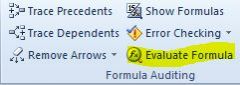
Evaluate a formula giving the wrong result:
=2+3*10 giving 32 and NOT 50 Highlight Formula Go to Formulas tab then Formula Auditing |
|
|
=COUNT(Price)
|
=COUNT(Price)
counts the number of something |
|
|
=MEDIAN(Price)
|
=MEDIAN(Price)
What is the middle number of this Name Range? |
|
|
=SUMIF(Price,F3)
|
=SUMIF(Price,F3)
Sum the items in the Price Range meeting the criteria in F3 |
|
|
=COUNTIF(Car_Type,F4)
|
=COUNTIF(Car_Type,F4)
Count the item in the Name range fitting the criteria in F4 |
|
|
To name a cell or range
|
To name a cell or range:
Highlight cell or range Click in Name Box Type Name Hit Enter Now this more meaningful Name can be used in Functions because it is already selected |
|
|
To edit, delete, or create names for a Name Region?
|
To edit, delete, or create names for a Named Region:
Ctrl + F3 |
|
|
Merging cells can cause later problems, so how do I handle
Titles, etc |
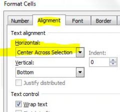
Merging cells can cause later problems,
so a better way to handle Titles, etc? Select a range of cells, then Ctrl + 1, then above illustration |
|
|
What are Ordering rule for borders?
|
Add Borders in this order:
1) Line 2) Color, 3) Border (add lines) |
|
|
Note:
Number Formatting is a Facade It sits on top of the number The number underneath the Number format may be different than the formatted number |
Using Currency or Accounting format
does not round a number To actually round a number, use the ROUND function = ROUND ( D1 , 1 ) to put the actual rounded number in calculations |
|
|
For example, the ROUND function can be used to reduce a value by a specific number of decimal places.
Unlike formatting options that allow you change the number of decimal places displayed, Excel's rounding functions actual alters the data in your worksheet |
The syntax for the ROUND function is:
= ROUND ( Number, Num_digits ) |
|
|
Ctrl + 1 with a chart does what?
|
Ctrl + 1
formatting chart area |
|
|
A chart title can be what is in a cell
|
Insert a Title,
then F2 to cell reference for a title |
|
|
To print only a selected area of a worksheet?
|
To print only a selected area of a worksheet
Select area Page Layout Set Print Area |
|
|
Alt+P+S+P
|
Alt+P+S+P
sets up the area to be printed after the area has been selected |
|
|
="AssumptionSheet"!B5
|
="AssumptionSheet"!B5
use data in another Worksheet other than the one currently on |
|
|
='Assumption Sheet'!B5
Why the single "'" |
='Assumption Sheet'!B5
has single ' because the Worksheet has a space in the name: Assumption Sheet NOT AssumptionSheet |
|

Why the [ ]
|
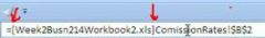
Brackets indicates going to another WorkBook
Note: using another workbook means the other workbook must be available the same way |
|
|
Note:
Enter enters data or formula, then moves down one cell Shift + Enter does the above, BUT moves up 1-cell |
Note:
Ctrl + Enter keeps you in the cell without moving down Tab to go right Shift + Tab to go left |
|
|
=IFERROR(C2/B2,"Review")
|
=IFERROR(C2/B2,"Review")
The general format is: =IFERROR(if formula is wrong, err msg is generated) |
|
.
|
|
|
|
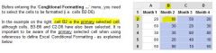
With Conditional Formatting
What does this do: =COLUMN()>$A2+1 |
Select the range you want to apply the formatting to, starting with a cell in row 2 on your example (as per attached)
Conditional formatting > New Rule > Use a formula =COLUMN()>$A2+1 Use the format button to choose the formatting to color blank cells in a region |
|
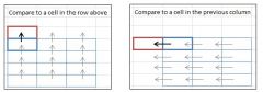
With Conditional Formating
The focus is writing a formula to compare a selection to the "red" cell |
Think in terms
of the desired condition comparison of the primary cell |
|
|
Advanced Filter can be used with a TRUE/FALSE formula
|
Again
Advanced Filter can be used with a TRUE/FALSE formula |
|
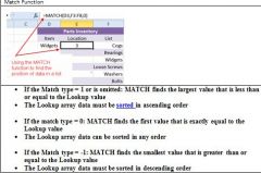
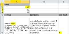
If Function
|

And again
|
|

.
|
And again
|
|
More efficient way to do a pseudo If Function
|

And again
|